Part 1 – Introduction to Hive

Hive is a data warehouse system built on top of Hadoop, allowing queries to be run through Hive Query Language (HiveQL), a language similar to SQL. Hive is best used where data structures are rigid and flat and where operations such as JOINs are needed i.e. operations that are simple in HiveQL, but very complex in standard Java MapReduce or Streaming.

In Hive, since you are using HDFS, large datasets can be manipulated across many nodes, while viewing data as a table and creating queries as if it were a database.

Issues with Hive

Hive is slowed by time spent communicating with MapReduce. However, many solutions exist which do not use MapReduce, such as Shark and Impala^[1].

Shark is fault tolerant like Hadoop – when one node fails, data is moved to another node so the whole query doesn’t fail. This is very useful for large datasets, where node failure is likely and queries take time.

Simple Hive Example

Take a simple file demoTable.txt which lists 4 famous Spanish League footballers of the 1950s/1960s:

PlayerID   PlayerName  Birth
1   Alfredo di Stefano  1926
2   Luis Suarez 1935
3   Ferenc Puskas   1927
4   Zoltan Czibor   1929

First create a table with a schema and load some data from HDFS into Hive:

CREATE TABLE demoTable (ID INT, PlayerName STRING, Birth INT)
ROW FORMAT DELIMITED FIELDS TERMINATED BY 't'
STORED AS TEXTFILE LOCATION 'demoTable.txt';

Now for a simple query to find players born before 1930:

INSERT OVERWRITE DIRECTORY 'demoResults'
SELECT PlayerName
FROM demoTable
WHERE Birth<1930;

This results in the following output, which can be found in the new directory demoResults:

Alfredo di Stefano
Ferenc Puskas
Zoltan Czibor

Key Differences between SQL and HiveQL

Hortonworks’ cheat sheet covers key differences between SQL and HiveQL as well as code for basic tasks^[2].

One notable example is that JOIN conditions have to be exact (unlike in SQL), however there are various ways around this e.g. WHERE clauses or CROSS JOINs can be used instead. Also, HiveQL is constantly being updated to remove as many of these restrictions as possible.

Part 2 – MovieLens Dataset

Lets look at the University of Minnesota’s MovieLens dataset^[3] and the “10M” dataset, which has 10,000,054 ratings and 95,580 tags applied to 10,681 movies by 71,567 users of the online movie recommender service MovieLens. Not all users provided both ratings and tags – 69,878 rated films (at least 20 each), while only 4,016 applied tags to films.

Format of Data

Original data is contained in 3 files – ratings.dat, tags.dat, movies.dat. For the following observations, a file genres.dat was added to help look more closely at individual genres.

Filename	Data Structure	Example
ratings.dat	UserID::MovieID::Rating::Timestamp	“1::122::5.0::838985046” represents User #1’s rating of 5.0 for Movie #122, which is 5.0. Using the file movies.dat we see that Movie #122 is the film “Boomerang” made in 1992.
movies.dat	MovieID::Title::Genres	The line for film 4973 is “4973::Amélie (Fabuleux destin d’Amélie Poulain, Le) (2001)::Comedy|Romance”, which is self-explanatory.
tags.dat	UserID::MovieID::Tag::Timestamp	The corresponding tag for User #15 is the line “15::4973::excellent!::1215184630” representing User #15’s tag of “excellent!” for Amélie
genres.dat	Genre	Alphabetic list of 18 genres from Action to Western.

The above format clearly suits the use of Hive and HiveQL. Firstly we have one wrinkle – fields are separated by a “::”, not recognised by Hive as a delimiter. However, with a short script in Python or R we can replace all occurrences of “::” with a tab (“\t”) in all input files.

Now we look at what’s actually in the files to see if there’s any issues. The following code shows the first 10 lines for movies.dat:

CREATE TABLE movies (MovieID INT, Title STRING, Genres String)
ROW FORMAT DELIMITED FIELDS TERMINATED BY 't'
STORED AS TEXTFILE LOCATION 'movies.dat';

SELECT * FROM movies LIMIT 10;

Which gives the following output:

1  Toy Story (1995)    Adventure|Animation|Children|Comedy|Fantasy
2   Jumanji (1995)  Adventure|Children|Fantasy
3   Grumpier Old Men (1995) Comedy|Romance
4   Waiting to Exhale (1995)    Comedy|Drama|Romance
5   Father of the Bride Part II (1995)  Comedy
6   Heat (1995) Action|Crime|Thriller
7   Sabrina (1995)  Comedy|Romance
8   Tom and Huck (1995) Adventure|Children
9   Sudden Death (1995) Action
10  GoldenEye (1995)    Action|Adventure|Thriller

As can be seen above, the title includes the film year e.g. the title for Toy Story is “Toy Story (1995)”, so it’s worth parsing the year into a separate record. Also this film has multiple genres, so we should use the Hive instr function to look at individual genres. No other issues are found in the other tables, tags or ratings.

The table full_data presented below, brings together all key components of the 2 tables ratings and movies, including film year which is extracted using Hive’s substr function:

CREATE TABLE full_data (UserID INT, Title STRING, Year INT, 
           Genres STRING, Rating DOUBLE);
INSERT OVERWRITE TABLE full_data
SELECT r.UserID,substr(m.Title,1,length(m.Title)-7),
       substr(m.Title,length(m.Title)-4,4), m.Genres,r.Rating
FROM ratings r
CROSS JOIN movies m
ON r.MovieID=m.MovieID;

This allows for us to run queries using Hive’s aggregate functions (e.g. avg, min, max, count) and make key observations that have an impact on marketing.

Note on Genres

As noted multiple genres appear in each film. To deal with this a JOIN of the tables full_data and genres using the condition instr(full_data.Genres, genres.genre) > 0 should work. However, pure JOINs have to be done with exact ON conditions. However, this is not so for CROSS JOINs:

SELECT g.genre,avg(f.rating)
FROM full_data f
CROSS JOIN genres g
WHERE instr(f.Genres,g.genre)>0
GROUP BY g.genre;

As CROSS JOINs produce more rows than a pure JOIN, this solution is quite inefficient. However Hive may be expanded in future to allow inexact conditions for pure JOINs.

Part 3 – Films

The following graphs show the average rating and number of films that were rated on an annual basis.

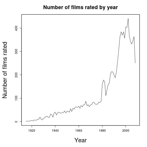This shows a rating preference towards older movies – only 3 times before 1978 is it below 3.6 and these years (1915,1919 and 1926) are in the silent era, while it is only very occasionally above 3.6 from 1978 on.

This is the trend that is expected. It would appear, based on the number of films rated by year, that older movies are only watched if they have a reputation for being good, while there is a wider range of quality when it comes to modern movies. For instance, only 12% of the films were made before 1960, about halfway through the film range chronologically.

Ratings

Below is a histogram of average film ratings, which shows a normal distribution spread from 1 to 5 with the centre somewhere between 3 and 4, and a Q-Q plot against normally distributed random variates.

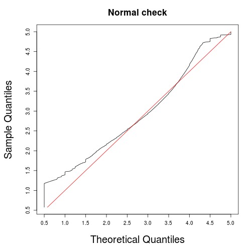The Q-Q plot shows this distribution similar to normal. This is the kind of distribution we expect, as the average rating is the average of many similarly distributed factors (e.g. overall quality, user interest, genre).

Part 4 – Users

Average Ratings by User

The following is a histogram of users’ average ratings, and a Q-Q plot which shows how close this is to a normal distribution.

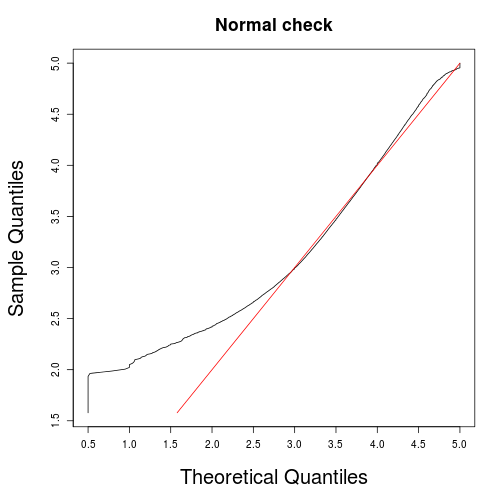Similar to the above case of average ratings by film, the distribution is shown to be similar to normal, where the average rating is the average of many similarly distributed factors (e.g. overall quality, user interest, genre).

Users’ Preferences by Year

The following 2 plots show the number of ratings by year of film and a frequency graph of the “average” year of user’s ratings, which give very similar distributions. The “average” year of a user’s ratings is defined as the mathematical average of the years of films they have rated, rounded to the nearest integer.

Both show a left skewed distribution, with 1995 being the year with most ratings and 1994 the most common user “average” year. This is the distribution we expect i.e. where most ratings are made on modern films but the number of ratings falls off as more immediately recent movies have not yet been viewed by everyone.

Users’ Preferences by Genre

Most users appear quite diverse in their tastes with 87% of users having rated films from 10 or more genres. However, many films come under multiple genres (e.g. The 1988 film “Who Framed Roger Rabbit?” comes under Adventure, Animation, Children, Comedy, Crime, Fantasy and Mystery) and only 37.5% of the films come under one genre.

Number of Ratings by User

The following is a frequency plot of the number of ratings.

The shape of this curve suggests that the number of users’ ratings follow a survival distribution. To check this we rephrase this as a survival problem and plot the function f, where f(n) is the number of users that have given at least n ratings:

Based on this curve, the number of films rated by a user appears to be indeed driven by a survival distribution. It would appear that the key driver behind the number of films rated by users is their interest in giving ratings which dies quite rapidly – while all 69,878 users rated at least 20 films, only 26,874 rated at least 100 movies and only 843 rated 1,000 movies.

Part 5 – Genres

The following scatter plots show the average rating and number of ratings by genre.

 

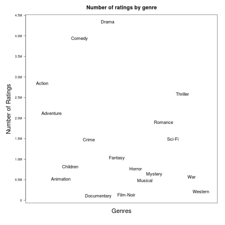
The most popular genre is Drama with 4.3 million films (43% of the dataset). While only 131,592 films fall under Film-Noir, this is the best rated film genre – perhaps linked to a propensity to rate films made before 1960 highly as 36.5% of film-noir films were made before 1960 (in contrast to 4.5% for Horror) the worst rated genre.

A closer look at these genres therefore appears prudent, particularly movie timings, as ratings for these genres would be expected to vary dramatically over time. Indeed the following graphs are the average ratings for each of these genres taken over 5 year intervals.

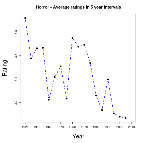In short users appear to prefer older Horror movies to modern Horror, while the difference isn’t as dramatic with Film-Noir. As well as standard recommender techniques (e.g. collaborative filtering based on users’ favourite films) it may be worth marketing vintage films to users with preferences for Horror.

References

1. ^ Shark: Real-time queries and analytics for big data, November 27, 2012
2. ^ Simple Hive ‘Cheat Sheet’ for SQL Users, August 20, 2013
3. ^ MovieLens Datasets