Weather Patterns Using Hadoop and R – Part 2

The first part of this post looked at data mining of world weather patterns such as cloud location and cloud coverage levels.

As these features describe aggregate values and ratios they are quite simple to evaluate with Hadoop, R and MapReduce Streaming. However for time dependant analytics, such as how long rainfall happens, additional issues need to be addressed.

Time Dependent Data Mining

Time based weather analytics focuses on weather at any location as time passes. This is done by extracting data using R so that Hadoop sorts data in the shuffle phase by weather station then time. However this is quite inefficient as, for any station, data is scattered across every file in the dataset.

Filtering down to 6 stations spread across the globe significantly reduces the data load for Hadoop’s shuffle phase, while there remains sufficient data to look at world weather and regional patterns.

The 6 stations are chosen across the globe:

  • Arctic and Antarctic – Danmarkshavn,Greenland and Base Belgrano II, an Argentinian run Antarctic weather station.
  • Mid Latitudes – Dublin Airport, Ireland and Christchurch, New Zealand.
  • Tropics – Khartoum, Sudan and La Paz, Bolivia.

The following R script brings this all together to form the Mapper:

# Mapper script
#! /usr/bin/env Rscript
stations <- c(" 4320", #Danmarkshavn
              " 3969", #Dublin Airport
              "62721", #Khartoum
              "85201", #La Paz
              "93890", #Christchurch
              "89674") #Base Belgrano II

#days in standard 365 day year
months <- c(31,28,31,30,31,30,31,31,30,31,30,31)
#days in year
#from 1981 to 1991, inclusive
years <- c(365,365,365,366,365,365,365,366,365,365,365)

con <- file("stdin", open = "r")
while (length(line <- readLines(con, n = 1, warn = FALSE)) > 0)
{
 if(length(stations[stations==substr(line,20,24)])!=0)
 {
    if(substr(line,1,2)=="84"
     | substr(line,1,2)=="88")
    {
     months[2] <- 29
    } else {
     months[2] <- 28
    }

   cat(sprintf("%s%5d%s%d\n",
 #land station synoptic code
 substr(line,20,24),                                
#time in number of hours since Jan 1, 1981 00:00
 sum(years[81:91<as.integer(substr(line,1,2))])*24
+sum(months[1:12<as.integer(substr(line,3,4))])*24
+(as.integer(substr(line,5,6))-1)*24
+as.integer(substr(line,7,8)),                
          substr(line,33,38),                          
 #precipitation level
 as.integer(as.numeric(substr(line,26,27))/10)
     ))
 }
}
close(con)

Using this script with an identity reducer data mining can be performed from the output in R, outside Hadoop. Note that a map-only job (achieved with the command line argument -D mapred.reduce.tasks=0) won’t shuffle the data, so an identity reducer is necessary for this task.

Results

When Precipitation Happens

As noted in the previous post, nimbostratus always occurs with precipitation. For stratus, 45% of the time this cloud appears precipitation develops before either the stratus disappears or 24 hours have passed. With other cloud types this rate ranges from 5% to 26%.

As mentioned before, high-level cloud types are not precipitation inducing so any data mining results relating to precipitation are meaningless[1].

How Long Precipitation Lasts

Within the 6 chosen stations nimbostratus precipitation lasts for up to 6 days, corresponding with the expectation that precipitation “is generally steady and prolonged”[1]. With stratus, precipitation can also last for up to 6 days, with cirrostratus for up to 4.5 days while for other cloud types the maximum is 3 days.

Cloud Development Patterns

Nimbostratus – follows altocumulus slightly more often than altostratus. May also form following occurrence of cirrus cloud cover and is roughly equally as likely to develop into altocumulus as altostratus.

Cirrus – at the 6 stations often develops into cirrostratus. Cirrostratus is known to form from “spreading and joining of cirrus clouds”[1].

Cumulus – at the chosen stations usually develops into stratocumulus or cumulonimbus. Indeed cumulonimbus is known to form from “upwardly mobile cumulus congestus clouds (thermals)”[1].

Stratocumulus – 31% of occurrences are followed by altocumulus. Indeed
altocumulus can form “by subdivision of a layer of stratocumulus”[2]. 27% of stratocumulus occurrences are followed by cumulus. Indeed “cumulus may originate from … stratocumulus”[3]. Also, 33% of stratocumulus occurrences are followed by stratus. This is line with the expectation that “stratus may develop from stratocumulus”[4].

Stratus – is more likely to develop into stratocumulus than no low cloud cover.

Conclusion

Again, data mining results compare quite well with established cloud facts and world weather satellite data, albeit this part of the study restricts itself to 6 land based locations.

The set of stations can be changed so that the trade-off between accuracy and time running Hadoop is optimal while various data analytics, such as regional weather effects, can be extracted. The main drawback is that this data mining involves re-running the MapReduce job each time the station list is changed.

References

  1. ^ a b c Common Cloud Names, Shapes, and Altitudes
  2. ^ Altocumulus
  3. ^ Cumulus
  4. ^ Stratus

Weather Patterns Using Hadoop and R – Part 1

In the post Cloud Weather Reporting with R and Hadoop the meaning of synoptic cloud data was not explored. This post looks at cloud patterns and their impact on world weather.

The cloud weather analytics covered mainly comprises aggregate frequency data (e.g. cloud location, coverage and precipitation types) and time series data (e.g. when precipitation happens and for how long). This post focusses on frequency data analytics, while the next post will focus on time dependant analytics.

Frequency Based Analytics

Frequency based properties are evaluated through MapReduce by extracting relevant weather data using the following R script as Mapper:

# Mapper script
#! /usr/bin/env Rscript

con <- file("stdin", open = "r")
while (length(line <- readLines(con, n = 1, warn = FALSE)) > 0)
{
 if(substr(line,9,9)=="1")
  cat(sprintf("%d%s%d\n",
      as.integer((abs(as.integer(substr(line,10,14))/2250)+1)/2),
      substr(line,33,38),
      as.integer(as.integer(substr(line,26,27))/10)))
 #output latitude, cloud types and precipitation level
 #latitude is coded as 0 for tropical, 1 for mid-latitudes, 2 for polar regions
}
close(con)

The Reducer script from a previous post gives counts for each combination of cloud type and precipitation level, from which most frequency based weather analytics can be derived. For example, stratocumulus frequency is the aggregate count of where the low cloud type code is 4,5 or 8, divided by the total number of reports in the dataset.

Ideally from a data mining perspective, error prone work such as interpretation of WMO codes and further data analytics can be done using an R script and, as this is outside Hadoop, can be tested and amended quickly.

Results

This data mining reveals a few properties of world weather, in addition to a few local weather patterns.

Location of Clouds

Nimbostratus is “common in middle latitudes”[1] – in the dataset 85% of nimbostratus occurrences are mid-latitude. Cumulonimbus is “common in tropics and temperate regions, rare at poles”[1], somewhat reflected in the dataset where 23% of occurrences of cumulonimbus are in tropical regions and 4% are in polar regions.

Likelihood of Precipitation

100% of occurrences of nimbostratus occur with precipitation, as WMO codes define precipitation bearing altostratus or altocumulus to be nimbostratus. Indeed nimbostratus is derived from ‘nimbus’, Latin for rain.

Conversely, high cloud types (cirrus, cirrostratus and cirrocumulus) generate no precipitation[1] so any perceived correlation with precipitation levels is meaningless. For remaining cloud types, precipitation occurrence levels range from 3% for cumulus to 38% for stratus. Indeed cumulus is associated with “generally no precipitation”[1].

Types of Precipitation

Cumulonimbus typically results in “Heavy downpours, hail”[1] – in the dataset 91% of precipitation associated with cumulonimbus is in the thunderstorm range. Indeed in the tropics, cumulonimbus often forms from hot weather through convection during monsoon season.

Conversely, nimbostratus is rarely seen with thunderstorms, more with “moderate to heavy rain or snow”[1] – 54% of nimbostratus occurrences happen with rain. Similarly, stratocumulus is usually accompanied by “occasional light rain, snow”[1] – 47% of cumulonimbus occurrences happen with rain.

Cloud Embedding

Cumulonimbus can be embedded with nimbostratus, and in such instances may result in heavy rain, but this is rare[2]. Indeed, further data mining reveals that only 5.9% of the occurrences of nimbostratus show this embedding.

Cloud Coverage Levels

The most significant cloud coverage comes from cirrus, stratocumulus and cumulus. For the dataset cirrus cloud cover is 22%, stratocumulus cloud cover is 24% and altocumulus cloud cover is 25%. This compares quite well to satellite data of 20 to 25% for cirrus[3], 25% for stratocumulus[2] and 20 to 25% for altocumulus[4].

Conclusion

The data mining results compare quite well with established cloud facts and world weather satellite data, particularly on location and coverage of clouds.

In the next post more complex data mining is presented i.e. time dependant analytics. For instance how to determine which clouds cause most prolonged rainfall? And how is this analytics done efficiently, given the amount of re-sorting of data involved?

References

  1. ^ a b c d e f Common Cloud Names, Shapes, and Altitudes
  2. ^ a Cloudwatching
  3. ^ Cirrus Clouds and Climate
  4. ^ Comparisons and analyses of aircraft and satellite observations for wintertime mixed-phase clouds

Marketers are targeting – what’s it to you?

The Way I See It - Mark Kolier

Targeting WSJ BN-DR632_CAMPAI_NS_20140714195702I hesitated to include what is nearly an entire article even from a venerated newspaper (or content provider?) such as the Wall Street Journal.   However since my partners and I continually discuss the nature of successful advertising, effective targeting is at the center of nearly all of our discussions – with and without clients in the room. 

Everyone knows that when online they are being targeted to some degree.   I feel the article below from Tuesday July 15, 2014, has a distinct point of view and goes far beyond what one might consider impartial reporting.

I don’t believe we have a single client that would ask us that we target less precisely, or charge them more money in order to not overly target prospective customers.

It is said that politics makes strange bedfellows. I will ask you to be the judge. Is the article below meant to scare or impress?…

View original post 1,144 more words

Recommenders Using the MovieLens Dataset

Recommendation Using Big Data

Traditionally, advertising is done through promotions such as billboards, newspapers and TV adverts. Although this remains an important kind of advertising, especially when aimed at people who don’t use the internet much, it can be costly and based on assumptions/generalisations about large groups of people.

However with Big Data it is possible to go deeper and market to individual users. Looking again at the MovieLens dataset from the post Evaluating Film User Behaviour with Hive it is possible to recommend movies to users based on their tastes using similar methods to those used by Amazon and Netflix.

Top Rated Movies

Looking again at the MovieLens dataset[1], and the “10M” dataset, a straightforward recommender can be built. Using the following Hive code, assuming the movies and ratings tables are defined as before, the top movies by average rating can be found:

CREATE TABLE f_m(movieID INT, avg_rating DOUBLE);
INSERT OVERWRITE TABLE f_m
SELECT MovieID,avg_rating
FROM
(
 --get average and number of ratings for each movie
 SELECT MovieID,avg(rating) AS avg_rating,count(rating) AS count_rating
 FROM ratings
 GROUP BY MovieID
) x
WHERE count_rating>=${hiveconf:sample_min}
ORDER BY avg_rating DESC
LIMIT ${hiveconf:topN};

--output movie titles by joining f_m and movies tables via movieID
INSERT OVERWRITE DIRECTORY '${hiveconf:OUTPUT}'
SELECT m.Title,f.avg_rating
FROM f_m f
JOIN movies m
ON f.MovieID=m.MovieID
ORDER BY f.avg_rating DESC;

The command line arguments -hiveconf topN=10 -hiveconf sample_min=20 set variables in Hive. topN is the number of movies in the final list and sample_min is the minimum number of ratings a movie has to have to consider its average rating. Single quotes e.g. ‘${hiveconf:OUTPUT}’ are used for string variables while the single quotes are left out for numerical variables.

This gives the following output:

Shawshank Redemption, The (1994)                4.457238321660348
Godfather, The (1972)                           4.415085293227011
Usual Suspects, The (1995)                      4.367142322253193
Schindler's List (1993)                         4.363482949916592
Sunset Blvd. (a.k.a. Sunset Boulevard) (1950)   4.321966205837174
Casablanca (1942)                               4.319740945070761
Rear Window (1954)                              4.316543909348442
Double Indemnity (1944)                         4.315439034540158
Seven Samurai (Shichinin no samurai) (1954)     4.314119283602851
Third Man, The (1949)                           4.313629402756509

User Based Recommendation

There are some obvious problems with the above algorithm, mainly that users’ tastes are not looked at. Another is that many users will have seen most of the movies in the top 10, if not all of them.

By accounting for movies already seen by individual users, this script gives each user their own list of top rated movies:

--extract list of unique userIDs
CREATE TABLE users(UserID INT);
INSERT OVERWRITE TABLE users
SELECT DISTINCT UserID
FROM ratings;

--table listing top rated movies by average rating
--excluding movies that aren't rated by enough users
CREATE TABLE f_m(movieID INT, avg_rating DOUBLE);
INSERT OVERWRITE TABLE f_m
SELECT MovieID,avg_rating
FROM
(
 --get average and number of ratings for each movie
 SELECT MovieID,avg(rating) AS avg_rating,count(rating) AS count_rating
 FROM ratings
 GROUP BY MovieID
) x
WHERE count_rating>=${hiveconf:sample_min}
ORDER BY avg_rating DESC;

--list of top 5 movies not seen by each user
CREATE TABLE Unseen(UserID INT,MovieID INT);
INSERT OVERWRITE TABLE Unseen
SELECT UserID,MovieID
FROM
(
 --get movie's ranking in UserID's list
 SELECT UserID,MovieID,row_number() OVER (PARTITION BY UserID ORDER BY avg_rating DESC) AS rank
 FROM
 (
  --generate table of movies in ufm not seen by user
  SELECT ufm.*
  FROM
  (
   --generate table of all possible user 
   --and movie combinations based on f_m
   SELECT *
   FROM users
   CROSS JOIN f_m
  ) ufm
  LEFT OUTER JOIN ratings r
  ON ufm.movieID=r.movieID AND ufm.userID=r.userID
  WHERE r.movieID IS NULL --exclude cases where user has seen movie
 ) x
) y
WHERE rank<=5;

--output movie titles by matching movieID with movie title
INSERT OVERWRITE DIRECTORY '${hiveconf:OUTPUT}'
SELECT U.UserID,m.Title
FROM Unseen U
JOIN movies m
ON U.MovieID=m.MovieID;

However the table f_m has 10,681 movies x 71,567 users ~ 764 million entries, which is unnecessarily large and inefficient. Eliminating as many poorly rated films as possible by adding the condition LIMIT ${hiveconf:sampleN} to the definition of f_m (after the line ORDER BY avg_rating DESC) controls the size of f_m and improves efficiency.

When generating a users’ list of top 5 unseen movies, if the value of sampleN is too low some users are recommended less than 5 movies. For this dataset a value of c.300 for sampleN is enough to sort this problem.

To fine-tune this further, genres and eras can be looked at. Defining the new table eras, where the table lists off all decades covered by the dataset, the following algorithm gives each user recommendations based on their favourite movie genres and decades:

--extract list of unique userIDs
CREATE TABLE users(UserID INT);
INSERT OVERWRITE TABLE users
SELECT DISTINCT UserID
FROM ratings;

--table listing of movies
--together with their average rating, genre and decade
--subject to a minimum ratings count
CREATE TABLE f_m(MovieID INT, Genre STRING, Decade INT, avg_rating DOUBLE);
INSERT OVERWRITE TABLE f_m
SELECT MovieID,genre,decade,avg_rating
FROM
(
 --extract main movie features
 --and get rating average and count
 SELECT MovieID,genre,decade,avg(rating) AS avg_rating,count(rating) AS count_rating
 FROM
 (
  --extract main movie features from table ratings
  --using movies and genres tables
  SELECT r.MovieID,g.genre,substr(m.Title,length(m.Title)-4,3) AS decade,r.rating
  FROM Ratings r
  JOIN movies m
  ON r.MovieID=m.MovieID
  CROSS JOIN genres g
  WHERE instr(m.Genres,g.genre)>0
 ) x
 GROUP BY MovieID,genre,decade
) y
WHERE count_rating>=${hiveconf:sample_min};

--table of each user's favourite combinations of genre and decade
CREATE TABLE Top5GE(UserID INT, Genre STRING, Decade INT);
INSERT OVERWRITE TABLE Top5GE
SELECT UserID,genre,decade
FROM
(
  --rank user's preferences
  --by number of movies in each genre and decade
 SELECT UserID,genre,decade,row_number() OVER (PARTITION BY UserID ORDER BY cge DESC) AS rank
 FROM
 (
  --count number of ratings
  --by user and combination of genre and decade
  SELECT UserID,genre,decade,count(rating) AS cge
  FROM
  (
   --extract main movie features from table ratings
   --using movies and genres tables
  SELECT r.UserID,g.genre,substr(m.Title,length(m.Title)-4,3) AS decade,r.rating
  FROM Ratings r
  JOIN movies m
  ON r.MovieID=m.MovieID
  CROSS JOIN genres g
  WHERE instr(m.Genres,g.genre)>0
   ) rmg
  GROUP BY UserID,genre,decade
 ) x
) rank_rmg
WHERE rank<=5;

--table of top rated movies
--for each possible combination of genre and decade
CREATE TABLE GenreEraMovies(movieID INT, Genre String, decade INT, avg_rating DOUBLE);
INSERT OVERWRITE TABLE GenreEraMovies
SELECT movieID,genre,decade,avg_rating
FROM
(
 --extract key movie features and match up to genres and decade
 --rank movies in genre/decade combination by average rating
 SELECT g.genre,e.decade,m.movieID,m.avg_rating,row_number() OVER (PARTITION by g.genre,e.decade order by m.avg_rating DESC) AS rank
 FROM genres g
 CROSS JOIN eras e
 JOIN f_m m
 ON m.genre=g.genre AND m.decade=e.decade
) x
WHERE rank<=${hiveconf:GEPool};

 --recommend the best movie in each user's
 --favourite combinations of genre and decade
CREATE TABLE Recom(UserID INT, MovieID INT);
INSERT OVERWRITE TABLE Recom
 --most movies have multiple genres
 --hence the DISTINCT keyword is used to remove duplicate recommendations
SELECT DISTINCT UserID,MovieID
FROM
(
 --rank movies by average rating
 --within each user's favourite combinations of genre and decade
 --excluding movies already seen by user
 SELECT tge.UserID,tge.MovieID,row_number() OVER (PARTITION BY tge.UserID,tge.genre,tge.decade ORDER BY tge.avg_rating DESC) AS rank
 FROM
 (
  --table that matches top rated movies
  --to each user's favourite combinations of genre and decade
  SELECT t.*,ge.MovieID,ge.avg_rating
  FROM GenreEraMovies ge
  JOIN Top5GE t
  ON ge.genre=t.genre AND ge.decade=t.decade
 ) tge
 --remove movies already seen by user
 LEFT OUTER JOIN ratings r
 ON tge.UserID=r.UserID AND tge.MovieID=r.MovieID
 WHERE r.UserID IS NULL
) x
WHERE rank=1;

--output movie titles by matching movieID with movie title
INSERT OVERWRITE DIRECTORY '${hiveconf:OUTPUT}'
SELECT R.UserID,m.Title
FROM Recom R
JOIN movies m
ON R.MovieID=m.MovieID;

Efficiency is controlled by the variable GEPool. After defining rank using the row_number() function, the condition WHERE rank<=${hiveconf:GEPool} limits the number of movies in this table. When GEPool is set to at least 50, users get at least 5 recommendations.

Collaborative Filtering

Collaborative filtering involves collecting information about user behaviour and making recommendations based on similarities between users.

Apache Mahout

Apache Mahout is a machine learning library in the Hadoop ecosystem that mainly includes algorithms for tasks such as recommendations, document clustering and document classification[2].

Mahout’s Item Based Recommender – Example

To illustrate the theory behind Mahout’s item based recommender, consider 4 users and 5 restaurants with the following user ratings:

ResTable

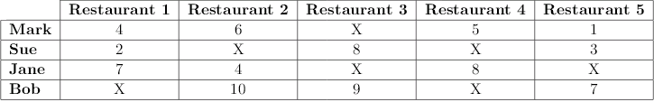
Ratings are integer based from 0 to 10, with untried restaurants marked with an X. Now consider recommending a new restaurant to Sue.

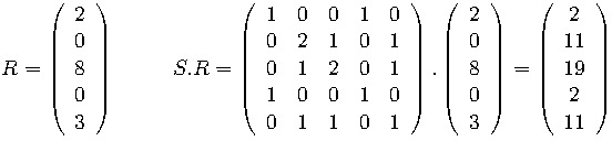
Mahout computes the similarity matrix for the restaurants, S, where S_ij is the number of users that rate both restaurants i and j positively (i.e. a rating of at least 6), while S_ii is the number of users that rate restaurant i positively.

S

This is then multiplied by the vector of Sue’s ratings, R (where untried restaurants are given a 0):

SxR

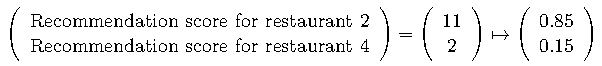
Ignoring restaurants Sue has already tried and normalising gives:

Recommend

This predicts Sue will much prefer Restaurant 2 to Restaurant 4.

Mahout’s Item Based Recommender – Analysis

As with any mathematical model there is no “correct” way to make recommendations, however it is possible to see why this approach makes sense. Focusing on the relevant rows of S and R in the computation of S.R

matmult1

this clearly recommends restaurants that are rated positively by users that also rate Sue’s favourite restaurants positively. Also the impact users’ ratings have on recommendation scores makes sense – a restaurant that is well rated by all users would get a high recommendation score, while a restaurant rated as 0 by all users gets a recommendation score of 0.

In practice S is a sparse matrix that is quite difficult to compute, as it involves a self join, however the latest editions of Mahout do not use MapReduce and are quite efficient.

Collaborative Filtering with MovieLens

An alternative to Mahout’s recommender is to compute the similarity matrix for movies in the MovieLens dataset. Then for any movie viewed by a user we can recommend films “often well rated with this movie”. The following Hive code does just that:

--get positively rated movies by UserID
CREATE TABLE sorted(userID INT,movieID INT);
INSERT OVERWRITE TABLE sorted
SELECT userID,movieID
FROM ratings
WHERE rating>=3.0; --condition for movie to be considered positively rated by user

--self-join positively rated movies
--identifying pairs of movies rated positively by the same user
INSERT OVERWRITE DIRECTORY '${hiveconf:OUTPUT}'
--recommend 5 movies for each movie
SELECT m1,m2
FROM
(
 --rank movie pairs by the number of users that rate both positively
 SELECT m1,m2,row_number() OVER (PARTITION BY m1 ORDER BY cnt DESC) AS rank
 FROM
 (
  --identify pairs of movies positively rated by the same user
  --and count how much this happens
  SELECT s1.movieID AS m1,s2.movieID AS m2,COUNT(*) AS cnt
  FROM sorted s1
  JOIN sorted s2
  ON s1.userID=s2.userID
  WHERE s1.movieIDs2.movieID
  GROUP BY s1.movieID,s2.movieID
 ) x
) y
WHERE rank<=5;

However this is quite inefficient, mainly because it uses a self join i.e. SELECT s1.movieID,s2.movieID,COUNT(*) AS count FROM sorted s1 JOIN sorted s2.

A better approach is to use the R function combn. For each user a list of movies they’ve rated positively is produced, from which all possible pairings of 2 movies is output. This can be done in Hive with a UDF defined in R, but using MapReduce is quicker with the following scripts:

#Mapper script to identify pairs of movies rated positively by the same user
#! /usr/bin/env Rscript

currentUserID <- ""
con <- file("stdin", open = "r")
while (length(line <- readLines(con, n = 1, warn = FALSE)) > 0)
{
 split <- strsplit(line,"\t")[[1]]
  if(currentUserID!=split[1])
  {
        if(currentUserID!="")
        {
         #remove last ":" from agg
         agg <- substr(agg,0,nchar(agg)-1)
         #parse individual movieIDs
         movies <- as.integer(strsplit(agg,",")[[1]])
          if(length(movies)>=2)
          {
           #output all possible pairings of movieIDs rated positively by same user
           write.table(t(combn(movies,2)),
                                   row.names = FALSE,col.names = FALSE,sep=",")
           write.table(t(combn(rev(movies),2)),
                                   row.names = FALSE,col.names = FALSE,sep=",")
          }
        }
   currentUserID <- split[1]
   agg <- ""
  }
  if(as.numeric(split[3])>=3.0) #condition to be considered rating as positive
   agg <- sprintf("%s%s,",agg,split[2]) #aggregate up movieIDs, to be parsed
}
close(con)

if(currentUserID!="")
{
 #remove last ":" from agg
 agg <- substr(agg,0,nchar(agg)-1)
 #parse individual movieIDs
 movies <- as.integer(strsplit(agg,",")[[1]])
   if(length(movies)>=2)
   {
         #output all possible pairings of movieIDs rated positively by same user
         write.table(t(combn(movies,2)),
                                 row.names = FALSE,col.names = FALSE,sep=",")
         write.table(t(combn(rev(movies),2)),
                                 row.names = FALSE,col.names = FALSE,sep=",")
        }
}
#Reducer script - for each movie outputs the 5 movies
#                 it is most often paired with by the Mapper
#! /usr/bin/env Rscript

currentMovieID <-  ""
current_pair <- ""
con <- file("stdin", open = "r")
while (length(line <- readLines(con, n = 1, warn = FALSE)) > 0)
{
 if(line!="")
 {
  if(current_pair!=line)
  {
        if(current_pair!="")
        {
         #add movieID to the vector top5
         #also add the amount of times it is paired with currentMovieID
         #to the vector count5
         top5 <- c(top5, strsplit(current_pair,",")[[1]][2])
         count5 <- c(count5,count)
        }
        if(strsplit(line,",")[[1]][1]!=currentMovieID)
        {
           if(currentMovieID!="") 
           {
                #sort count5, rearrange top5 based on this sort
                #and keep the first 5 elements of these vectors
                top5 <- top5[order(count5,decreasing=TRUE)][1:min(length(top5),5)]
                count5 <- sort(count5,decreasing=TRUE)[1: min(length(top5),5)]
                #output recommended MovieIDs
                cat(sprintf("%s\t%s\t%d",currentMovieID,top5,count5),sep="\n")
           }
         top5 <- c()
         count5 <- c()
         currentMovieID <- strsplit(line,",")[[1]][1]
        }
   current_pair <- line
   count <- 0
  }
  count <- count + 1
 }
}
close(con)

if(current_pair!="")
{
 #sort count5, rearrange top5 based on this sort
 #and keep the first 5 elements of these vectors
 top5 <- c(top5, strsplit(current_pair,",")[[1]][2])
 count5 <- c(count5,count)
 top5 <- top5[order(count5,decreasing=TRUE)][1:5]
 count5 <- sort(count5,decreasing=TRUE)[1:5]
 #output recommended MovieIDs
 cat(sprintf("%s\t%s\t%d",currentMovieID,top5,count5),sep="\n")
}

This outputs pairs of MovieIDs, which can be converted into pairs of movie titles with a simple Hive script, using the table movies. Overall this algorithm’s efficiency is due to
combn being a vectorised function i.e. the speed of the calculation of combn(movies,2) is constant regardless of the size of the vector movies.

Looking at the results, one problem can be seen when looking at what gets recommended to users that have watched Toy Story:

Toy Story (1995)   Dead Poets Society (1989)
Toy Story (1995)    Nightmare Before Christmas, The (1993)
Toy Story (1995)    Phenomenon (1996)
Toy Story (1995)    Raiders of the Lost Ark (Indiana Jones and the Raiders of the Lost Ark) (1981)
Toy Story (1995)    This Is Spinal Tap (1984)

Watching a children’s movie results in potentially inappropriate recommendations. A simplistic solution would be to have movies match by genre. However, given that most movies are under multiple genres, this doesn’t remove enough suspect matches to actually deal with the issue.

A better solution is to add rules to the code e.g. for each children’s movie only other children’s movies are recommended. Given that genre data and ratings data are in 2 different tables the best approach is, before running the MapReduce job, to start with the following Hive script to match up each rating with movie title and key genre:

INSERT OVERWRITE DIRECTORY '${hiveconf:OUTPUT}'
SELECT r.UserID,m.MovieID,if(instr(m.Genres,"Children")>0,"Children",
           if(instr(m.Genres,"Documentary")>0,"Documentary","Standard"))
FROM ratings r
JOIN movies m
ON r.MovieID=m.MovieID
WHERE r.rating>=3.0
ORDER BY r.UserID;

Then some changes are also needed in the R scripts that make up the MapReduce Job. Firstly the line that aggregates movies, agg <- sprintf("%s%s,",agg,split[2]), must be changed as many movie titles will contain the character “,”, interfering with the use of the strsplit function to separate out movie titles. Instances of “,” are replaced with “:”, which isn’t in any movie title, while the line genres <- sprintf("%s%s:",agg,split[3]) is added to include a treatment of genres.

Secondly the variable filter is defined so only pairs of movies passing genre rules are matched i.e. for children’s movies only other children’s movies are recommended and for documentaries only other documentaries are recommended. The following code does that:

filter <- (genres[1,]==genres[2,] | genres[1,]=="Standard")
          movies1 <- matrix(c(movies[,1][filter],movies[,2][filter]),ncol=2)
          filter <- (genres[1,]==genres[2,] | genres[2,]=="Standard")
          movies2 <- matrix(c(movies[,2][filter],movies[,1][filter]),ncol=2)

          write.table(movies1,row.names = FALSE, col.names = FALSE,
                                                  sep=":", quote = FALSE)
          write.table(movies2,row.names = FALSE, col.names = FALSE,
                                                  sep=":", quote = FALSE)

Already we see an improvement, with the following recommendations for Toy Story:

Toy Story (1995) Finding Nemo (2003)
Toy Story (1995) Goonies, The (1985)
Toy Story (1995) Harry Potter and the Prisoner of Azkaban (2004)
Toy Story (1995) Nanny McPhee (2005)
Toy Story (1995) Rescuers Down Under, The (1990)

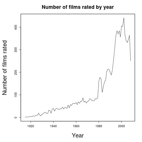
Children’s movies from different eras, such as The Goonies, and that might not have necessarily been considered by users previously, are recommended under this system. However vintage movies, such as Vertigo, will not necessarily be paired with other vintage movies given the dataset’s bias towards modern movies:

Vertigo (1958) 12 Monkeys (Twelve Monkeys) (1995)
Vertigo (1958) Being John Malkovich (1999)
Vertigo (1958) Godfather, The (1972)
Vertigo (1958) Indiana Jones and the Temple of Doom (1984)
Vertigo (1958) Toy Story (1995)

Simply changing the filter variable to

filter <- ((substr(movies[,1],nchar(movies[,1])-4,nchar(movies[,1])-2)
                                 ==substr(movies[,2],nchar(movies[,2])-4,nchar(movies[,2])-2))
                                 & (genres[1,]==genres[2,] | genres[1,]=="Standard"))

adds a match by decade. Now Vertigo gets the following recommendations:

Vertigo (1958) Diary of Anne Frank, The (1959)
Vertigo (1958) Kiss Me Kate (1953)
Vertigo (1958) People Will Talk (1951)
Vertigo (1958) Show Boat (1951)
Vertigo (1958) Suddenly, Last Summer (1959)

Conclusion

These are just a sample of many approaches that can be used to recommend. In practice, weighted combination of specific methods can be used, fined-tuned by the research of the post Evaluating Film User Behaviour with Hive . The more data, the better, so it should come as no surprise that companies reputed to have the most accurate recommenders are the likes of Amazon, Google, and Netflix.

Movie data such as country, language or director and user data such as sex or age is only a sample of what can be added for more accurate recommendations. Social networking data can also be used to recommend based on friends’ tastes and matching similar users.

The scale of this approach can be quite large and costly – while some pieces of code from the Netflix Prize were implemented by Netflix, the final winner wasn’t used as engineering costs outweighed accuracy benefits[3].

References

  1. ^ MovieLens Datasets
  2. ^ What is Apache
    Mahout
  3. ^ Netflix Recommendations: Beyond the 5 stars (Part 1) , April 6, 2012

Evaluating Film User Behaviour with Hive

Part 1 – Introduction to Hive

Hive is a data warehouse system built on top of Hadoop, allowing queries to be run through Hive Query Language (HiveQL), a language similar to SQL. Hive is best used where data structures are rigid and flat and where operations such as JOINs are needed i.e. operations that are simple in HiveQL, but very complex in standard Java MapReduce or Streaming.

In Hive, since you are using HDFS, large datasets can be manipulated across many nodes, while viewing data as a table and creating queries as if it were a database.

Issues with Hive

Hive is slowed by time spent communicating with MapReduce. However, many solutions exist which do not use MapReduce, such as Shark and Impala[1].

Shark is fault tolerant like Hadoop – when one node fails, data is moved to another node so the whole query doesn’t fail. This is very useful for large datasets, where node failure is likely and queries take time.

Simple Hive Example

Take a simple file demoTable.txt which lists 4 famous Spanish League footballers of the 1950s/1960s:

PlayerID   PlayerName  Birth
1   Alfredo di Stefano  1926
2   Luis Suarez 1935
3   Ferenc Puskas   1927
4   Zoltan Czibor   1929

First create a table with a schema and load some data from HDFS into Hive:

CREATE TABLE demoTable (ID INT, PlayerName STRING, Birth INT)
ROW FORMAT DELIMITED FIELDS TERMINATED BY 't'
STORED AS TEXTFILE LOCATION 'demoTable.txt';

Now for a simple query to find players born before 1930:

INSERT OVERWRITE DIRECTORY 'demoResults'
SELECT PlayerName
FROM demoTable
WHERE Birth<1930;

This results in the following output, which can be found in the new directory demoResults:

Alfredo di Stefano
Ferenc Puskas
Zoltan Czibor

Key Differences between SQL and HiveQL

Hortonworks’ cheat sheet covers key differences between SQL and HiveQL as well as code for basic tasks[2].

One notable example is that JOIN conditions have to be exact (unlike in SQL), however there are various ways around this e.g. WHERE clauses or CROSS JOINs can be used instead. Also, HiveQL is constantly being updated to remove as many of these restrictions as possible.

Part 2 – MovieLens Dataset

Lets look at the University of Minnesota’s MovieLens dataset[3] and the “10M” dataset, which has 10,000,054 ratings and 95,580 tags applied to 10,681 movies by 71,567 users of the online movie recommender service MovieLens. Not all users provided both ratings and tags – 69,878 rated films (at least 20 each), while only 4,016 applied tags to films.

Format of Data

Original data is contained in 3 files – ratings.dat, tags.dat, movies.dat. For the following observations, a file genres.dat was added to help look more closely at individual genres.

Filename Data Structure Example
ratings.dat UserID::MovieID::Rating::Timestamp “1::122::5.0::838985046” represents User #1’s rating of 5.0 for Movie #122, which is 5.0. Using the file movies.dat we see that Movie #122 is the film “Boomerang” made in 1992.
movies.dat MovieID::Title::Genres The line for film 4973 is “4973::Amélie (Fabuleux destin d’Amélie Poulain, Le) (2001)::Comedy|Romance”, which is self-explanatory.
tags.dat UserID::MovieID::Tag::Timestamp The corresponding tag for User #15 is the line “15::4973::excellent!::1215184630” representing User #15’s tag of “excellent!” for Amélie
genres.dat Genre Alphabetic list of 18 genres from Action to Western.

The above format clearly suits the use of Hive and HiveQL. Firstly we have one wrinkle – fields are separated by a “::”, not recognised by Hive as a delimiter. However, with a short script in Python or R we can replace all occurrences of “::” with a tab (“\t”) in all input files.

Now we look at what’s actually in the files to see if there’s any issues. The following code shows the first 10 lines for movies.dat:

CREATE TABLE movies (MovieID INT, Title STRING, Genres String)
ROW FORMAT DELIMITED FIELDS TERMINATED BY 't'
STORED AS TEXTFILE LOCATION 'movies.dat';

SELECT * FROM movies LIMIT 10;

Which gives the following output:

1  Toy Story (1995)    Adventure|Animation|Children|Comedy|Fantasy
2   Jumanji (1995)  Adventure|Children|Fantasy
3   Grumpier Old Men (1995) Comedy|Romance
4   Waiting to Exhale (1995)    Comedy|Drama|Romance
5   Father of the Bride Part II (1995)  Comedy
6   Heat (1995) Action|Crime|Thriller
7   Sabrina (1995)  Comedy|Romance
8   Tom and Huck (1995) Adventure|Children
9   Sudden Death (1995) Action
10  GoldenEye (1995)    Action|Adventure|Thriller

As can be seen above, the title includes the film year e.g. the title for Toy Story is “Toy Story (1995)”, so it’s worth parsing the year into a separate record. Also this film has multiple genres, so we should use the Hive instr function to look at individual genres. No other issues are found in the other tables, tags or ratings.

The table full_data presented below, brings together all key components of the 2 tables ratings and movies, including film year which is extracted using Hive’s substr function:

CREATE TABLE full_data (UserID INT, Title STRING, Year INT, 
           Genres STRING, Rating DOUBLE);
INSERT OVERWRITE TABLE full_data
SELECT r.UserID,substr(m.Title,1,length(m.Title)-7),
       substr(m.Title,length(m.Title)-4,4), m.Genres,r.Rating
FROM ratings r
CROSS JOIN movies m
ON r.MovieID=m.MovieID;

This allows for us to run queries using Hive’s aggregate functions (e.g. avg, min, max, count) and make key observations that have an impact on marketing.

Note on Genres

As noted multiple genres appear in each film. To deal with this a JOIN of the tables full_data and genres using the condition instr(full_data.Genres, genres.genre) > 0 should work. However, pure JOINs have to be done with exact ON conditions. However, this is not so for CROSS JOINs:

SELECT g.genre,avg(f.rating)
FROM full_data f
CROSS JOIN genres g
WHERE instr(f.Genres,g.genre)>0
GROUP BY g.genre;

As CROSS JOINs produce more rows than a pure JOIN, this solution is quite inefficient. However Hive may be expanded in future to allow inexact conditions for pure JOINs.

Part 3 – Films

The following graphs show the average rating and number of films that were rated on an annual basis.

avgratingbyyear NumFilmsByYear

This shows a rating preference towards older movies – only 3 times before 1978 is it below 3.6 and these years (1915,1919 and 1926) are in the silent era, while it is only very occasionally above 3.6 from 1978 on.

This is the trend that is expected. It would appear, based on the number of films rated by year, that older movies are only watched if they have a reputation for being good, while there is a wider range of quality when it comes to modern movies. For instance, only 12% of the films were made before 1960, about halfway through the film range chronologically.

Ratings

Below is a histogram of average film ratings, which shows a normal distribution spread from 1 to 5 with the centre somewhere between 3 and 4, and a Q-Q plot against normally distributed random variates.

Film_ratings_full Film_ratings_full-NORM_CHECK

The Q-Q plot shows this distribution similar to normal. This is the kind of distribution we expect, as the average rating is the average of many similarly distributed factors (e.g. overall quality, user interest, genre).

Part 4 – Users

Average Ratings by User

The following is a histogram of users’ average ratings, and a Q-Q plot which shows how close this is to a normal distribution.

UserID_avg_rating UserID_avg_rating-NORM_CHECK

Similar to the above case of average ratings by film, the distribution is shown to be similar to normal, where the average rating is the average of many similarly distributed factors (e.g. overall quality, user interest, genre).

Users’ Preferences by Year

The following 2 plots show the number of ratings by year of film and a frequency graph of the “average” year of user’s ratings, which give very similar distributions. The “average” year of a user’s ratings is defined as the mathematical average of the years of films they have rated, rounded to the nearest integer.

numfilmsbyyear UserID_avg_year

Both show a left skewed distribution, with 1995 being the year with most ratings and 1994 the most common user “average” year. This is the distribution we expect i.e. where most ratings are made on modern films but the number of ratings falls off as more immediately recent movies have not yet been viewed by everyone.

Users’ Preferences by Genre

Most users appear quite diverse in their tastes with 87% of users having rated films from 10 or more genres. However, many films come under multiple genres (e.g. The 1988 film “Who Framed Roger Rabbit?” comes under Adventure, Animation, Children, Comedy, Crime, Fantasy and Mystery) and only 37.5% of the films come under one genre.

Number of Ratings by User

The following is a frequency plot of the number of ratings.
UserIDRatingNumFULL

The shape of this curve suggests that the number of users’ ratings follow a survival distribution. To check this we rephrase this as a survival problem and plot the function f, where f(n) is the number of users that have given at least n ratings:
UserIDRatingNumFULLCumulative

Based on this curve, the number of films rated by a user appears to be indeed driven by a survival distribution. It would appear that the key driver behind the number of films rated by users is their interest in giving ratings which dies quite rapidly – while all 69,878 users rated at least 20 films, only 26,874 rated at least 100 movies and only 843 rated 1,000 movies.

Part 5 – Genres

The following scatter plots show the average rating and number of ratings by genre.
numratingsbygenre
 
avgratingbygenre

The most popular genre is Drama with 4.3 million films (43% of the dataset). While only 131,592 films fall under Film-Noir, this is the best rated film genre – perhaps linked to a propensity to rate films made before 1960 highly as 36.5% of film-noir films were made before 1960 (in contrast to 4.5% for Horror) the worst rated genre.

A closer look at these genres therefore appears prudent, particularly movie timings, as ratings for these genres would be expected to vary dramatically over time. Indeed the following graphs are the average ratings for each of these genres taken over 5 year intervals.

FilmNoir_avg_ratings_5years Horror_avg_ratings_5years

In short users appear to prefer older Horror movies to modern Horror, while the difference isn’t as dramatic with Film-Noir. As well as standard recommender techniques (e.g. collaborative filtering based on users’ favourite films) it may be worth marketing vintage films to users with preferences for Horror.

References

  1. ^ Shark: Real-time queries and analytics for big data, November 27, 2012
  2. ^ Simple Hive ‘Cheat Sheet’ for SQL Users, August 20, 2013
  3. ^ MovieLens Datasets

Cloud Weather Reporting with R and Hadoop

Part 1 – Introduction to Hadoop

Hadoop is a software platform to manage and mine large datasets, by allowing users of commodity servers access massively parallel computing.

Structure of Hadoop

Hadoop has 2 main components – HDFS and MapReduce.

HDFS manages data storage and administration. HDFS divides files into blocks of data, typically 64MB in size, then stores them across a cluster of data nodes. Any data task can then be performed over many large files stored on many machines. This eliminates many traditional limits on data processing including allowing for dramatic increases in data capacity.

MapReduce is Hadoop’s main data processing framework, written in Java. To see how it works, imagine counting Irish authors in a library. MapReduce would delegate shelves to team members (i.e. divide data into blocks) who count Irish authors within their assigned shelves (the Mapper process). The workers then get together to add up their results (the Reducer process).

The Hadoop Ecosytem

As Java MapReduce can be complex, Apache have added projects to simplify its use. Streaming runs MapReduce scripts languages other than Java, Hive runs SQL-like queries in Hadoop while Pig performs SQL-like operations in a procedural language that users of R and Python might be more comfortable with.

These are only some of the projects available and companies continue to find other ways to simplify the use of Hadoop such as online tools like Amazon’s AWS service, which includes S3 file storage (a similar file system to HDFS) and their Elastic MapReduce platform.

Benefits of Hadoop

Hadoop enables a solution that is:

  • Scalable – New nodes can be added as needed without changing many features of data loading or job construction. Also the scalability is linear i.e. doubling the amount of clusters halves the time spent on work.
  • Cost Effective – Hadoop brings massively parallel computing to commodity servers with a sizeable decrease in the cost per unit.
  • Flexible – Hadoop can absorb any type of data, structured or not, from any number of sources, enabling deeper analyses than any one system can give.
  • Fault Tolerant – When a node is lost, work is redirected to another node in the cluster.

Issues with Hadoop

  • Speed – Hadoop is not fast for small datasets and to be avoided for time critical processes. Hadoop is best for large tasks where time isn’t a constraint such as end-of-day reports or scanning historicals.
  • Complexity – Hadoop is still complex to use and requires specialised programming skills, which can eat into the data cost savings Hadoop offers. However Hadoop is constantly expanding with projects to simplify its use.
  • Not a Replacement for SQL – Hadoop is best suited to processing vast stores of accumulated data while more traditional relational databases are better suited for items like day-to-day transactional records.

The above issues are being tackled as Hadoop develops and, in particular, Impala’s developers are aiming to make Impala very usable for more traditional database tasks such as business intelligence applications.

Examples of Commercial Uses of Hadoop

Hadoop can be used for automated marketing, fraud prevention and detection, analysis of social network sites and relationships, in-store behaviour analysis in retail and marketing via 3G based on mobile device location. Hadoop is used by many leading-edge Internet companies such as Google, Yahoo, Facebook and Amazon.

While Hadoop is slow for small datasets, data needs are growing rapidly at many firms. Tynt, a company that observes web visitor behaviour, processes on average 20 billion internet user events per month. Before using Hadoop, additional MySQL databases were added weekly. Now, with Hadoop, additional storage requirements are managed more easily.[1]

Twitter have found that they can’t reliably write to a traditional hard drive given the sheer amount of data it stores – 12TB per day as of September 2010[2]. In addition, they use Pig scripts as SQL can’t perform operations of the scale they require[3].

Part 2 – The Cloud Weather Dataset

Data is downloaded from the website of the Carbon Dioxide Information Analysis Center[4], showing cloud and illuminescence data from land weather stations and ocean observation decks around the globe.

Using the Data

Files cover the period 1 December 1981 to 30 November 1991 with 2 files per month (1 for land observations and 1 for ocean observations) totalling 240 files (10 years x 12 months x 2 files). This is a perfect example where using Hadoop is helpful for data mining.

Each file has a number of weather observations – each line is a 56 character weather report. As per the documentation associated with the dataset[5], key items within each report are as follows:

Character Explanation Example/Usage
Characters 1-8 Year, Month, Day, Hour 6pm on the 13th March, 1986 is coded as 86031318.
Character 9 Sky Brightness Indicator A value of 1 means the sky is bright enough for the report to be used, as it has passed an illuminescence criterion.
Characters 10-14 Latitude (x100) The latitude for Dublin Airport is 53°25’N, represented by 5343 (53.43 degrees).
Characters 15-19 Longtitude (x100) The longtitude for Dublin Airport is 6°18’W = 353°42’E, represented by 35375 (353.75 degrees).
Characters 20-24 Synoptic Station Number The synoptic station number for Dublin Airport is 03969.
Characters 26-27 Present Weather (pw) Indicates whether precipitation is present:

  • pw<40,
    pw=76 or
    pw=78                no precipitation or fog
  • 40<=pw<50        fog
  • 50<=pw<60        drizzle
  • 60<=pw<70        rain
  • 70<=pw=80        storm.
Characters 33-34 Low Cloud Type Indicates if stratus, stratocumulus, cumulus or cumulonimbus are present.
Characters 35-36 Middle Cloud Type Indicates if nimbostratus, altostratus or altocumulus are present.
Characters 37-38 High Cloud Type Indicates if cirrostratus, cirrus, cirrocumulus or dense cirrus are present.

Part 3 – Using R on Cloud Weather Dataset

Using the documentation and R’s substr function we can write code in R to extract key values. For example, to extract the date we could run the following code:

year <- as.integer(sprintf("19%s",substr(line,1,2)))
month <- as.integer(substr(line,3,4))
day <- as.integer(substr(line,5,6))

Using R with Hadoop Streaming

Although the Cloud Weather dataset is large (c. 2GB) it wouldn’t be considered as “Big Data”, and indeed software such as PostgresSQL[6] and Pandas[7] exist that can handle such datasets. Nevertheless, this is a good example for illustrating how to use Hadoop.

An example of a program we might want to run is to evaluate the percentage of reports that pass the illuminescence criterion. If we were using one file, this could be done using the following R script:

#! /usr/bin/env Rscript

#initialise variables
pass <- fail <- 0
con <- file("stdin", open = "r")

#read input line by line
while (length(line <- readLines(con, n = 1, warn = FALSE)) > 0)
{
 #read the relevant illuminescence data
 sky_brightness <- as.integer(substr(line,9,9))

 #evaluate illuminescence data and increment relevant pass/fail variable
 if(sky_brightness==1) pass <- pass + 1
 if(sky_brightness==0) fail <- fail + 1
}
close(con)

pass_ratio <- pass/(pass+fail)

#output
cat(sprintf("pass_ratio=t%fn",pass_ratio))

However, as files get larger, the R script gets slower. This is for similar reasons to why opening very large files in standard text editors is slow. Hadoop can handle such a task in a better way as HDFS adapts to changes in data structure and can take multiple files as input.

In MapReduce, we can form a solution similar to the example of counting Irish authors that we had in Part 1. In effect what we are trying is the equivalent of a SQL GROUP BY and SUM query to get totals for pass and fail. We do so with the following steps:

  1. Map – the “master” node takes input and distributes it to “slave” nodes, which are all assigned a Mapper. Each Mapper counts the values of pass and fail, which are output back to the master node. The output is tab separated and of the form “keytvalue” where “passt189” means illuminescence was met 189 times at the slave node.
  2. Shuffle – Map output is sorted by key. This is, in effect, the “GROUP BY” part of the step, following which only one pass through data is required to get the total values of pass and fail.
  3. Reduce – as with the Map phase, the Shuffled output is assigned to Reducers which parse values of pass and fail and aggregate these values up, from which the ratio of “passes” can be derived.

The following is the R script for the Mapper:

#! /usr/bin/env Rscript

#initialise variables
pass <- 0
fail <- 0
con <- file("stdin", open = "r")

#read input line by line
while (length(line <- readLines(con, n = 1, warn = FALSE)) > 0)
{
 #read the relevant illuminescence data
 sky_brightness <- as.integer(substr(line,9,9))

 #evaluate illuminescence data and increment relevant pass/fail variable
 if(sky_brightness==1) pass <- pass + 1
 if(sky_brightness==0) fail <- fail + 1
}
close(con)

#intermediate output
cat(sprintf("passt%dn",pass))
cat(sprintf("failt%dn",fail))

Before presenting the Reducer script, it is instructive to first look at the effect of the Shuffle phase. For instance suppose Map output (in key, value pairs) is as follows:

pass    4535
fail    1037
pass    2357
fail    123
pass    1256
fail    479
pass    980
fail    1000

Then after the Shuffle phase it is sorted as follows:

pass    4535
pass    2357
pass    1256
pass    980
fail    1037
fail    123
fail    479
fail    1000

Now all the pass and fail keys are together in the output. The totals of pass and fail can be added up without additional variables in our script, with the following procedure:

1. Set count=0
2. When key="fail", increment count by value associated with key
3. After parsing final "fail" key, output value of count
4. Reset count=0 and repeat steps 1-3 for lines where key="pass"

This is the Reducer procedure as an R script:

#! /usr/bin/env Rscript

#control variable to check if key has changed since last line
old_key <- ""
con <- file("stdin", open = "r")

#loop through Map output line by line
while (length(line <- readLines(con, n = 1, warn = FALSE)) > 0)
{
 split <- strsplit(line,"t")[[1]]

 #parse out key and value
 key <- split[1]
 value <- as.integer(split[2])

 #check if key has changed since last line, or if we're at start
 if(old_key!=key)
 {
  #if not at start of file output latest key count.
  if(old_key!="") cat(sprintf("%s=%dn",old_key,count))

  #reset count and update old_key
  count <- 0
  old_key <- key
 }
 count <- count + value
}
close(con)

#at end of file add last key count
if(old_key!="") cat(sprintf("%s=%dn",old_key,count))

The above map/reduce scripting concept can be used for other cloud features e.g. getting a frequency histogram of lower cloud types is possible with the following Mapper script:

#! /usr/bin/env Rscript

C_l <- (-1:11)*0
con <- file("stdin", open = "r")

#read input line by line
while (length(line <- readLines(con, n = 1, warn = FALSE)) > 0)
{
 sky_brightness <- as.integer(substr(line,9,9))
 low_cloud_type <- as.integer(substr(line,33,34))
 if(sky_brightness==1) C_l[low_cloud_type+2] <- C_l[low_cloud_type+2] + 1
}
close(con)

#intermediate output
cat(sprintf("C_l%dt%d",-1:11,C_l),sep="n")

and then using the same Reducer script from the previous example. The output of this MapReduce job can be read in R using the strsplit function to parse the values vector C_l, from which a histogram can be generated.

Part 4 – Overview of Cloud Weather Dataset

Exporting files to Amazon S3, Amazon’s Elastic MapReduce platform (which includes Streaming) offers the opportunity to use the above approach to make several observations.

There were a total of 138,886,548 weather reports in the 10 year period, 124,164,607 made from land and 14,721,941 made from ocean, which corresponds with the documentation. In terms of the illuminescence criterion, 27.2% of all land reports and 24.6% of ocean reports failed it, showing little variability between land and ocean reports.

Histograms of Cloud Features

A good way to check the results of our Hadoop streaming programs is to recreate the frequency plots of cloud types, cloud base height and total cloud cover that are in the documentation. The following is the frequency of total cloud cover on land, derived using R with Hadoop Streaming, compared to the relevant histogram in documentation:

PrecipLandN nland

We note that cases of missing cloud data (Total Cloud Cover of -1) and obscured skies (Total Cloud Cover of 9) were removed before publishing online and hence are not in the graph on the left. Otherwise the 2 graphs are proportionally similar. We see the same result for all other cloud features, indicating the MapReduce algorithms are working correctly.

Factors that Affect Cloud Types and Features

  • Latitude – As we go towards the poles, cloud types become less varied and more reports of missing cloud data are seen. Histograms of cloud features on opposite ends of the globe tend to be similar, particularly as we get closer to the poles. The following are frequency plots of high cloud types on land, at equatorial regions and at both poles:

    -15to0-LandC_h 0to15-LandC_h
    -90to-75-LandC_h 75to90-LandC_h
  • Land or Ocean – On ocean, cloud types show a lot more variability than on land. Also errors in data are more frequent on ocean than on land. This is most profound when looking at lower cloud types globally:

    LandC_l OceanC_l

    Similarly, total cloud cover and lower cloud base height tend to be in the higher octaves on ocean than on land. Again, errors in data for these cloud features are more frequent on ocean than on land.

Part 5 – Occurrence of Precipitation

Monthly Occurrence of Precipitation Globally by Latitude

Using the documentation and the values of month, present_weather and latitude it is possible to show monthly precipitation trends.

In summary, the results show the expected seasonal influence on precipitation levels between latitudes of 30 to 75 degrees North or South, where precipitation happens more often during winter months than in summer. The following shows precipitation levels between 45 and 60 degrees of latitude in both hemispheres:

45to60 -60to-45

However, more interesting results are seen in tropical and arctic/antarctic regions. In tropical regions, more precipitation is seen during summer months, which appears to be because of the effect convectional rain has on precipitation levels[8]. Indeed the following plots of monthly precipitation in equatorial regions show this trend:

0to15 -15to0

In arctic/antarctic regions, there is no clear seasonal effect on precipitation levels:

75to90 -90to-75

Precipitation Across the United Kingdom & Ireland

Weather reports include land station and ocean deck codes, allowing filtering on a more local level. For example, all land weather stations in the United Kingdom and Ireland have the prefix “03” in their 5 digit number e.g. Dublin Airport is represented by the code 03969 and London Gatwick is represented by the code 03776.

In R the if clause if(grepl(“03”, stat_deck)) filters stations in the United Kingdom and Ireland, where stat_deck <- as.integer(substr(line,20,24) is the weather station code. The following plot of UK precipitation levels shows a similar trend to that seen globally in the region between latitudes of 45 to 60 degrees North.
UK&Ire

References

  1. ^ Cloudera Helps Tynt Customers Get a Clear Picture of Reader Interest, January 12, 2011
  2. ^ Twitter passes MySpace in traffic, adds 12TB of data per day, September 29, 2010
  3. ^ Hadoop at Twitter, April 8, 2010
  4. ^ Carbon Dioxide Information Analysis Center – Data on Synoptic Cloud Reports from Ships and Land Stations Over the Globe, 1982-1991
  5. ^ Edited Synoptic Cloud Reports from Ships and Land Stations Over the Globe, 1982-1991
  6. ^ Python Data Analysis Library
  7. ^ PostgreSQL
  8. ^ Rainfall Patterns