Part 1 – Introduction to Hadoop
Hadoop is a software platform to manage and mine large datasets, by allowing users of commodity servers access massively parallel computing.
Structure of Hadoop
Hadoop has 2 main components – HDFS and MapReduce.
HDFS manages data storage and administration. HDFS divides files into blocks of data, typically 64MB in size, then stores them across a cluster of data nodes. Any data task can then be performed over many large files stored on many machines. This eliminates many traditional limits on data processing including allowing for dramatic increases in data capacity.
MapReduce is Hadoop’s main data processing framework, written in Java. To see how it works, imagine counting Irish authors in a library. MapReduce would delegate shelves to team members (i.e. divide data into blocks) who count Irish authors within their assigned shelves (the Mapper process). The workers then get together to add up their results (the Reducer process).
The Hadoop Ecosytem
As Java MapReduce can be complex, Apache have added projects to simplify its use. Streaming runs MapReduce scripts languages other than Java, Hive runs SQL-like queries in Hadoop while Pig performs SQL-like operations in a procedural language that users of R and Python might be more comfortable with.
These are only some of the projects available and companies continue to find other ways to simplify the use of Hadoop such as online tools like Amazon’s AWS service, which includes S3 file storage (a similar file system to HDFS) and their Elastic MapReduce platform.
Benefits of Hadoop
Hadoop enables a solution that is:
- Scalable – New nodes can be added as needed without changing many features of data loading or job construction. Also the scalability is linear i.e. doubling the amount of clusters halves the time spent on work.
- Cost Effective – Hadoop brings massively parallel computing to commodity servers with a sizeable decrease in the cost per unit.
- Flexible – Hadoop can absorb any type of data, structured or not, from any number of sources, enabling deeper analyses than any one system can give.
- Fault Tolerant – When a node is lost, work is redirected to another node in the cluster.
Issues with Hadoop
- Speed – Hadoop is not fast for small datasets and to be avoided for time critical processes. Hadoop is best for large tasks where time isn’t a constraint such as end-of-day reports or scanning historicals.
- Complexity – Hadoop is still complex to use and requires specialised programming skills, which can eat into the data cost savings Hadoop offers. However Hadoop is constantly expanding with projects to simplify its use.
- Not a Replacement for SQL – Hadoop is best suited to processing vast stores of accumulated data while more traditional relational databases are better suited for items like day-to-day transactional records.
The above issues are being tackled as Hadoop develops and, in particular, Impala’s developers are aiming to make Impala very usable for more traditional database tasks such as business intelligence applications.
Examples of Commercial Uses of Hadoop
Hadoop can be used for automated marketing, fraud prevention and detection, analysis of social network sites and relationships, in-store behaviour analysis in retail and marketing via 3G based on mobile device location. Hadoop is used by many leading-edge Internet companies such as Google, Yahoo, Facebook and Amazon.
While Hadoop is slow for small datasets, data needs are growing rapidly at many firms. Tynt, a company that observes web visitor behaviour, processes on average 20 billion internet user events per month. Before using Hadoop, additional MySQL databases were added weekly. Now, with Hadoop, additional storage requirements are managed more easily.[1]
Twitter have found that they can’t reliably write to a traditional hard drive given the sheer amount of data it stores – 12TB per day as of September 2010[2]. In addition, they use Pig scripts as SQL can’t perform operations of the scale they require[3].
Part 2 – The Cloud Weather Dataset
Data is downloaded from the website of the Carbon Dioxide Information Analysis Center[4], showing cloud and illuminescence data from land weather stations and ocean observation decks around the globe.
Using the Data
Files cover the period 1 December 1981 to 30 November 1991 with 2 files per month (1 for land observations and 1 for ocean observations) totalling 240 files (10 years x 12 months x 2 files). This is a perfect example where using Hadoop is helpful for data mining.
Each file has a number of weather observations – each line is a 56 character weather report. As per the documentation associated with the dataset[5], key items within each report are as follows:
| Character | Explanation | Example/Usage |
| Characters 1-8 | Year, Month, Day, Hour | 6pm on the 13th March, 1986 is coded as 86031318. |
| Character 9 | Sky Brightness Indicator | A value of 1 means the sky is bright enough for the report to be used, as it has passed an illuminescence criterion. |
| Characters 10-14 | Latitude (x100) | The latitude for Dublin Airport is 53°25’N, represented by 5343 (53.43 degrees). |
| Characters 15-19 | Longtitude (x100) | The longtitude for Dublin Airport is 6°18’W = 353°42’E, represented by 35375 (353.75 degrees). |
| Characters 20-24 | Synoptic Station Number | The synoptic station number for Dublin Airport is 03969. |
| Characters 26-27 | Present Weather (pw) |
Indicates whether precipitation is present:
|
| Characters 33-34 | Low Cloud Type | Indicates if stratus, stratocumulus, cumulus or cumulonimbus are present. |
| Characters 35-36 | Middle Cloud Type | Indicates if nimbostratus, altostratus or altocumulus are present. |
| Characters 37-38 | High Cloud Type | Indicates if cirrostratus, cirrus, cirrocumulus or dense cirrus are present. |
Part 3 – Using R on Cloud Weather Dataset
Using the documentation and R’s substr function we can write code in R to extract key values. For example, to extract the date we could run the following code:
year <- as.integer(sprintf("19%s",substr(line,1,2)))
month <- as.integer(substr(line,3,4))
day <- as.integer(substr(line,5,6))
Using R with Hadoop Streaming
Although the Cloud Weather dataset is large (c. 2GB) it wouldn’t be considered as “Big Data”, and indeed software such as PostgresSQL[6] and Pandas[7] exist that can handle such datasets. Nevertheless, this is a good example for illustrating how to use Hadoop.
An example of a program we might want to run is to evaluate the percentage of reports that pass the illuminescence criterion. If we were using one file, this could be done using the following R script:
#! /usr/bin/env Rscript

#initialise variables
pass <- fail <- 0
con <- file("stdin", open = "r")

#read input line by line
while (length(line <- readLines(con, n = 1, warn = FALSE)) > 0)
{
 #read the relevant illuminescence data
 sky_brightness <- as.integer(substr(line,9,9))

 #evaluate illuminescence data and increment relevant pass/fail variable
 if(sky_brightness==1) pass <- pass + 1
 if(sky_brightness==0) fail <- fail + 1
}
close(con)

pass_ratio <- pass/(pass+fail)

#output
cat(sprintf("pass_ratio=t%fn",pass_ratio))
However, as files get larger, the R script gets slower. This is for similar reasons to why opening very large files in standard text editors is slow. Hadoop can handle such a task in a better way as HDFS adapts to changes in data structure and can take multiple files as input.
In MapReduce, we can form a solution similar to the example of counting Irish authors that we had in Part 1. In effect what we are trying is the equivalent of a SQL GROUP BY and SUM query to get totals for pass and fail. We do so with the following steps:
- Map – the “master” node takes input and distributes it to “slave” nodes, which are all assigned a Mapper. Each Mapper counts the values of pass and fail, which are output back to the master node. The output is tab separated and of the form “keytvalue” where “passt189” means illuminescence was met 189 times at the slave node.
- Shuffle – Map output is sorted by key. This is, in effect, the “GROUP BY” part of the step, following which only one pass through data is required to get the total values of pass and fail.
- Reduce – as with the Map phase, the Shuffled output is assigned to Reducers which parse values of pass and fail and aggregate these values up, from which the ratio of “passes” can be derived.
The following is the R script for the Mapper:
#! /usr/bin/env Rscript

#initialise variables
pass <- 0
fail <- 0
con <- file("stdin", open = "r")

#read input line by line
while (length(line <- readLines(con, n = 1, warn = FALSE)) > 0)
{
 #read the relevant illuminescence data
 sky_brightness <- as.integer(substr(line,9,9))

 #evaluate illuminescence data and increment relevant pass/fail variable
 if(sky_brightness==1) pass <- pass + 1
 if(sky_brightness==0) fail <- fail + 1
}
close(con)

#intermediate output
cat(sprintf("passt%dn",pass))
cat(sprintf("failt%dn",fail))
Before presenting the Reducer script, it is instructive to first look at the effect of the Shuffle phase. For instance suppose Map output (in key, value pairs) is as follows:
pass    4535
fail    1037
pass    2357
fail    123
pass    1256
fail    479
pass    980
fail    1000
Then after the Shuffle phase it is sorted as follows:
pass    4535
pass    2357
pass    1256
pass    980
fail    1037
fail    123
fail    479
fail    1000
Now all the pass and fail keys are together in the output. The totals of pass and fail can be added up without additional variables in our script, with the following procedure:
1. Set count=0
2. When key="fail", increment count by value associated with key
3. After parsing final "fail" key, output value of count
4. Reset count=0 and repeat steps 1-3 for lines where key="pass"
This is the Reducer procedure as an R script:
#! /usr/bin/env Rscript

#control variable to check if key has changed since last line
old_key <- ""
con <- file("stdin", open = "r")

#loop through Map output line by line
while (length(line <- readLines(con, n = 1, warn = FALSE)) > 0)
{
 split <- strsplit(line,"t")[[1]]

 #parse out key and value
 key <- split[1]
 value <- as.integer(split[2])

 #check if key has changed since last line, or if we're at start
 if(old_key!=key)
 {
  #if not at start of file output latest key count.
  if(old_key!="") cat(sprintf("%s=%dn",old_key,count))

  #reset count and update old_key
  count <- 0
  old_key <- key
 }
 count <- count + value
}
close(con)

#at end of file add last key count
if(old_key!="") cat(sprintf("%s=%dn",old_key,count))
The above map/reduce scripting concept can be used for other cloud features e.g. getting a frequency histogram of lower cloud types is possible with the following Mapper script:
#! /usr/bin/env Rscript

C_l <- (-1:11)*0
con <- file("stdin", open = "r")

#read input line by line
while (length(line <- readLines(con, n = 1, warn = FALSE)) > 0)
{
 sky_brightness <- as.integer(substr(line,9,9))
 low_cloud_type <- as.integer(substr(line,33,34))
 if(sky_brightness==1) C_l[low_cloud_type+2] <- C_l[low_cloud_type+2] + 1
}
close(con)

#intermediate output
cat(sprintf("C_l%dt%d",-1:11,C_l),sep="n")
and then using the same Reducer script from the previous example. The output of this MapReduce job can be read in R using the strsplit function to parse the values vector C_l, from which a histogram can be generated.
Part 4 – Overview of Cloud Weather Dataset
Exporting files to Amazon S3, Amazon’s Elastic MapReduce platform (which includes Streaming) offers the opportunity to use the above approach to make several observations.
There were a total of 138,886,548 weather reports in the 10 year period, 124,164,607 made from land and 14,721,941 made from ocean, which corresponds with the documentation. In terms of the illuminescence criterion, 27.2% of all land reports and 24.6% of ocean reports failed it, showing little variability between land and ocean reports.
Histograms of Cloud Features
A good way to check the results of our Hadoop streaming programs is to recreate the frequency plots of cloud types, cloud base height and total cloud cover that are in the documentation. The following is the frequency of total cloud cover on land, derived using R with Hadoop Streaming, compared to the relevant histogram in documentation:

|

|
We note that cases of missing cloud data (Total Cloud Cover of -1) and obscured skies (Total Cloud Cover of 9) were removed before publishing online and hence are not in the graph on the left. Otherwise the 2 graphs are proportionally similar. We see the same result for all other cloud features, indicating the MapReduce algorithms are working correctly.
Factors that Affect Cloud Types and Features
-
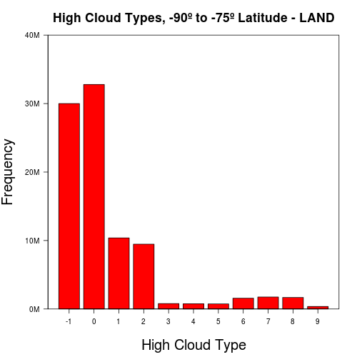
Latitude – As we go towards the poles, cloud types become less varied and more reports of missing cloud data are seen. Histograms of cloud features on opposite ends of the globe tend to be similar, particularly as we get closer to the poles. The following are frequency plots of high cloud types on land, at equatorial regions and at both poles:
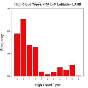
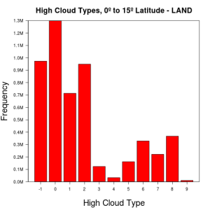

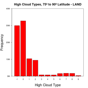
-
Land or Ocean – On ocean, cloud types show a lot more variability than on land. Also errors in data are more frequent on ocean than on land. This is most profound when looking at lower cloud types globally:
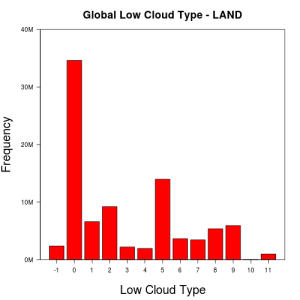
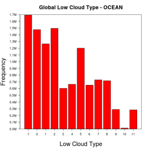
Similarly, total cloud cover and lower cloud base height tend to be in the higher octaves on ocean than on land. Again, errors in data for these cloud features are more frequent on ocean than on land.


Part 5 – Occurrence of Precipitation
Monthly Occurrence of Precipitation Globally by Latitude
Using the documentation and the values of month, present_weather and latitude it is possible to show monthly precipitation trends.
In summary, the results show the expected seasonal influence on precipitation levels between latitudes of 30 to 75 degrees North or South, where precipitation happens more often during winter months than in summer. The following shows precipitation levels between 45 and 60 degrees of latitude in both hemispheres:

|

|
However, more interesting results are seen in tropical and arctic/antarctic regions. In tropical regions, more precipitation is seen during summer months, which appears to be because of the effect convectional rain has on precipitation levels[8]. Indeed the following plots of monthly precipitation in equatorial regions show this trend:

|

|
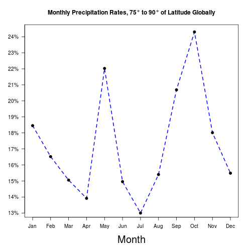
In arctic/antarctic regions, there is no clear seasonal effect on precipitation levels:
|

|
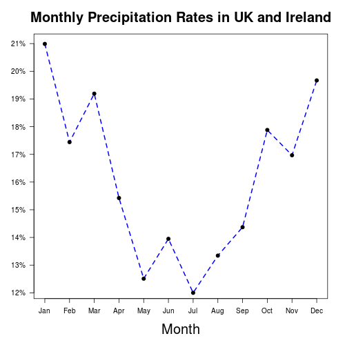
Precipitation Across the United Kingdom & Ireland
Weather reports include land station and ocean deck codes, allowing filtering on a more local level. For example, all land weather stations in the United Kingdom and Ireland have the prefix “03” in their 5 digit number e.g. Dublin Airport is represented by the code 03969 and London Gatwick is represented by the code 03776.
In R the if clause if(grepl(“03”, stat_deck)) filters stations in the United Kingdom and Ireland, where stat_deck <- as.integer(substr(line,20,24) is the weather station code. The following plot of UK precipitation levels shows a similar trend to that seen globally in the region between latitudes of 45 to 60 degrees North.
References
- ^ Cloudera Helps Tynt Customers Get a Clear Picture of Reader Interest, January 12, 2011
- ^ Twitter passes MySpace in traffic, adds 12TB of data per day, September 29, 2010
- ^ Hadoop at Twitter, April 8, 2010
- ^ Carbon Dioxide Information Analysis Center – Data on Synoptic Cloud Reports from Ships and Land Stations Over the Globe, 1982-1991
- ^ Edited Synoptic Cloud Reports from Ships and Land Stations Over the Globe, 1982-1991
- ^ Python Data Analysis Library
- ^ PostgreSQL
- ^ Rainfall Patterns


You must be logged in to post a comment.